By Lewis Bishop
The force is strong with this one…
If you’ve not heard of Power Query and/or you’re wondering why I’m banging my Power Query drum right now, check out our previous blog Power Query: Feel The Force.
Long story short, Power Query is a tool that is already embedded in Excel and Power BI, and is, like, amazing at automating processes for importing, merging, transforming and manipulating data. You don’t need to learn how to code, or write SQL, or talk to JSON, or crawl through HTM-hell to get quick, impactful results.
My previous blog sang Power Query’s praises in general, avoiding technical specifics to appeal to folks out there who aren’t the most comfortable with high-fallutin’ technobabble and give them a new hope. (If it wasn’t already clear, we quite like Star Wars at Productle.)
In this blog, we’re going to put Power Query through a few paces. We’ll keep things nice and simple, crisp and clear, and will show off the (nearly) unlimited power of Power Query – without having to turn to the dark side, which is, of course, techno mumbo jumbo. *shudders*
Combining multiple spreadsheets into one file The moment I fell in love with Power Query came when I learned how to automatically pull multiple spreadsheets into one file at the push of a button.
I had a daily task of importing 20+ webforms into a CRM. These webforms all had the same layout, and contained a mixture of donations, registrations, sponsorship income and various supporter data. I had to download them separately as csv files, format each document one at a time, then import all those files into the CRM. It was manual. It was time-consuming. It was as boring as working on a moisture farm on Tatooine.
Then a wise old sage with magical powers (translation: Grant the Analyst who sat at the desk next to mine) showed me a different path. He taught me to put all those different unformatted csv files straight into one folder, point Power Query at that folder and then format and combine everything in that folder with a touch of the Refresh button. What had taken hours would now take minutes.
In one fell stroke I became more powerful than you could possibly imagine. Here’s how you can too! The guidance here uses the current Microsoft 365 version of Excel; other versions may vary a little.
Using a folder as a source:
Create a folder for all those files that you want to combine. This is your Source Folder.
Put all the files you want to combine in your Source Folder. These files must be of the same type (e.g., csv, xls) and have the same column layout.
Open Excel and click on the Data tab.
Click on Get Data and select From File.
Select From Folder.
Browse to the folder that contains the files you want to import, in our case, your Source Folder.
Select the folder and click on OK.
Select the Combine drop-down and click on Combine & Transform Data.
Select the tab on the files that you want to import (Sheet1 if you haven’t renamed anything) and click on OK.
GIF showing using a folder as a source.
You should now be looking at Power Query Editor, with all the rows from your multiple files sitting in one table. ISN’T IT BEAUTIFUL?!? Well stop admiring your handiwork, because you’ll need to do some transformations to format the data.
Applied Steps Whatever transformations you perform here will be saved in Applied Steps (to the right of this Editor screen), and it is these Applied Steps that will be repeated whenever you click the Refresh button in the future!
What you need to do to the data in these Applied Steps will vary depending upon the type of files you’ve saved in your Source Folder (e.g., csv or xls). Power Query is smart and will usually apply some steps for you, but it also gives you the freedom to apply transformations unique to your requirements.
Here are the top 5 the most common transformations you’ll need:
Promote Headers: This step is often one of the first. The way your data was combined may have left you with column names like Source.Name, Column1 and Column2, and your first row may now contain your column names. Just click on the Home tab, select Row 1, and from the ribbon above click Use First Row as Headers. Next you’ll see that your column names are correct and Promoted Headers appears as an Applied Step.
Change Type: This step allows you to dictate what type of data is in each column (e.g., the Amount column is filled with currency type data). Click on the Home tab, select the column in question, select Data Type from the ribbon and choose whichever type you like.
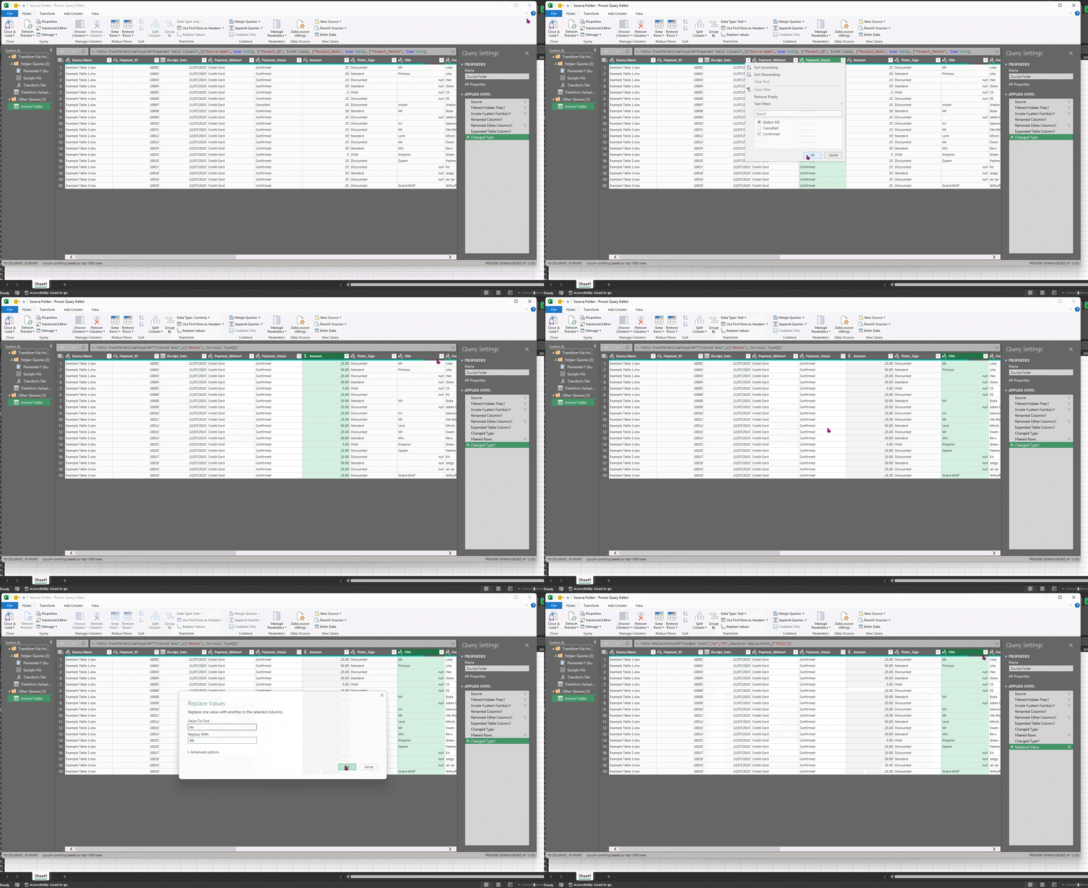
Filter Rows: This step allows you to filter rows based on specific criteria (e.g., only show payment lines with the status of Confirmed). Like in standard Excel, use the drop-down arrow in the column header and select your filter criteria.
Replace Values: This step allows you to set up the automatic replacement of recurring words and terms (e.g., customers write multiple variations of “Mr” in the title column, you want to set up a rule to replace “Mister”, “mr” and “MR” with “Mr”). Click on the Home tab, right-click the header of the column you want to replace values in, select Replace Values, and enter the relevant values in Value To Find and Replace With. You can add as many of these as you like!
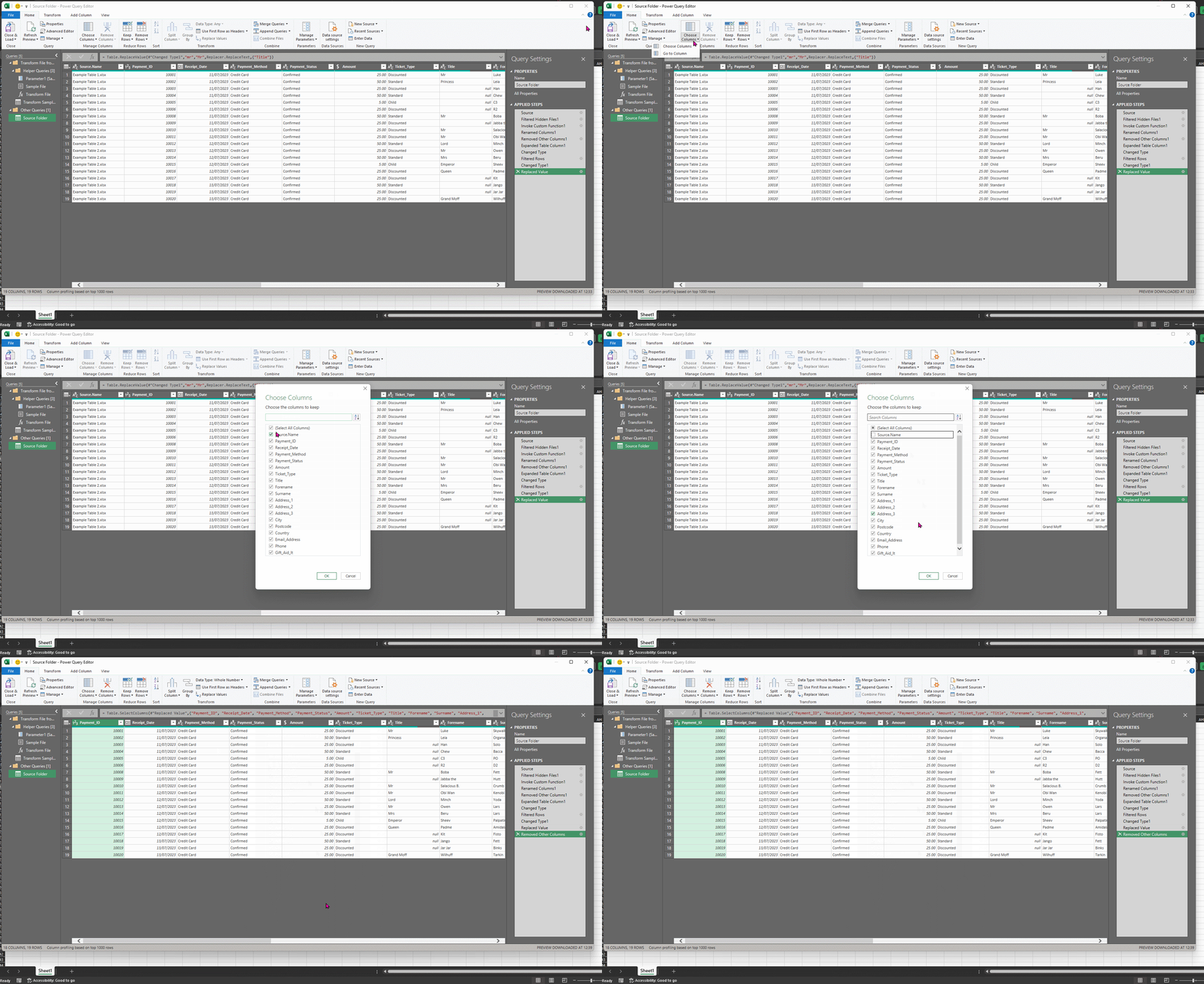
Remove Columns: This step allows you to remove columns that you don’t need from your dataset/final output. Combining different files together often creates a new first column informing you of which individual file that row came from. If you don’t need that, or any other column, just click on the Home tab, select Choose Columns and untick whichever columns you don’t want in your output.
GIF showing Filter Rows and Replace Values
GIF showing Choose Columns
Close & Load Once you’ve transformed your data with the Applied Steps, click on the Home tab and click Close & Load on the ribbon. This will close the Power Query Editor and will take you back to standard Excel, where – TA-DAH! – a table has appeared. It’s so pretty, it’s formatted exactly how you wanted it, and it has the data from every separate file from your Source Folder in one beautiful table.
GIF showing Close and Load instructions.
But you have not yet begun to reap the bountiful rewards of this process. Save this file anywhere but your Source Folder. Now the next time you add a new file to your Source Folder, all you need to do is open the processor file that you have created and…
Refresh the Data First Open Excel and click on the Data tab, then Click on Refresh All.
GIF showing Refresh instructions.
Aaaaaand that’s it! You will now see that your table has automatically formatted and added the rows from any new files you’ve saved in your Source Folder.
Congratulations, young padawan. Your training is complete.
May the force be with you. Always.


